How to Make a Dynamic Calendar in LibreOffice Calc

Step-by-Step Guide: How to Make a Dynamic Calendar in LibreOffice Calc

This guide outlines the complete process for creating an editable, dynamic calendar template in LibreOffice Calc that automatically updates when you select a new month or year.

Inspiration from

---

Step 1: Initial Page & Document Setup

1. Create a New Spreadsheet:
   • Open LibreOffice Calc.
   • Select File -> New -> Spreadsheet from the menu.
2. Configure Page Settings and Print Area:
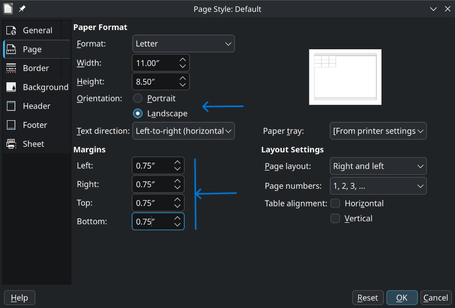
   • Go to File -> Print Preview-> Format Page
   • In the Page tab:
     • Select paper format (e.g., US Letter or A4).
     • Set orientation to Landscape.
     • Set desired margins (e.g., 0.75" on all sides).
     • Click OK. Dashed lines will appear indicating the printable area boundaries.
3. Remove Headers and Footers:
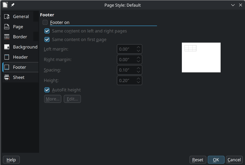
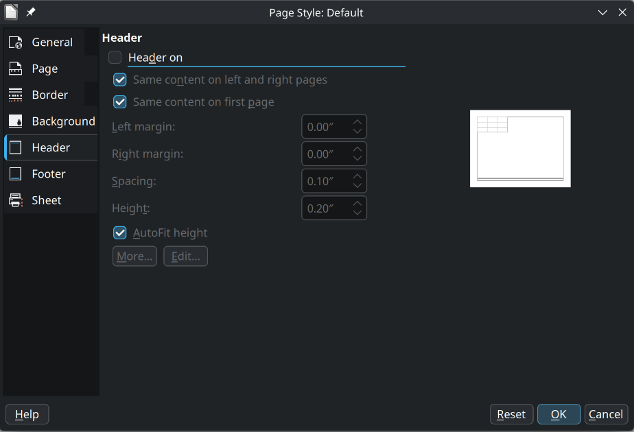
   • Go to File -> Print Prevew -> Format Page
   • In the Header tab, uncheck Header on.
   • In the Footer tab, uncheck Footer on.
   • Click OK.

Step 2: Set Up Worksheet Tabs

1. Double-click the existing sheet tab (Sheet1) and rename it to Month Calendar.
   • Add a second sheet and name it Settings.
2. Populate Month List:
   • Switch to the Settings sheet.
   • In Column A (cells A1 to A12), type the names of the 12 months sequentially (e.g., January through December).
3. Add Data Validity (Dropdown List):
   • Switch back to the Month Calendar sheet.
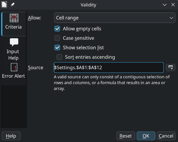
   • Select cell A1.
   • Go to Data -> Validity…
   • In the Criteria tab:
     • Under Allow, choose Cell Range.
     • In the Source field, enter: $Settings.$A$1:$A$12
   • Click OK. Cell A1 now features a drop-down arrow to select any month.

---

Step 3: Layout Header & Adjust Dimensions

1. Format Month Header:
   • Merge the top cells (e.g., A1:C1) to provide space for the month title.
   • Increase font size (e.g., size 40).
   • Left Align
2. Calculate & Set Column Widths:
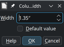
   • Determine width per column based on paper width and margins: Open your calculator application. For me it’s (11-20.75)/7=1.3571. Note: only use the first 2 decimals, LibreOffice will round the number anyway. *(Example for 11” US Letter Landscape with 0.75” margins: $(11 - 1.5) / 7 = 1.3571" \approx 1.35"$.)
   • Select headers for the first 7 columns (A through G).
   • Right-click and choose Column Width….
   • Enter your calculated width (e.g., 1.35") and click OK. (The print boundary dashed line should align right after Column G).

1. Add Year and Day Names:

   • In cell G1, enter a year manually (e.g., 2026) or use the dynamic formula:

     =YEAR(TODAY())

   • Format G1 with the same font and size as the month header.
   • In row 2 (cells A2:G2), enter the weekday names (e.g., Sunday through Saturday).

---

Step 4: Configure Dynamic Calendar Formulas

1. Calculate Starting Date of Calendar Grid:

   • To make the grid dynamic, cell A3 (first cell of week 1) must calculate the first date shown in the calendar grid (which may fall in the previous month if the 1st of the month isn’t a Sunday): 111116

     =DATE(G1,MATCH(A1,$Settings.A1:A12,0),1) - (WEEKDAY(DATE(G1,MATCH(A1,$Settings.A1:A12,0),1)) - 1)

     • DATE(G1, MATCH(A1, $Settings.A1:A12, 0), 1) retrieves the 1st day of the selected month/year.
     • WEEKDAY(...) calculates the day index (1 = Sunday, 7 = Saturday).
     • Subtracting WEEKDAY(...) - 1 offsets the calendar back to the preceding Sunday.
2. Populate Grid Formulas:
   • Week 1 Row (Row 3):
     • Cell B3: =A3+1
     • Cell C3: =B3+1 (drag/copy across to G3).
   • Row 4: Leave empty (used as event/note space under Week 1).
   • Week 2 Row (Row 5):
     • Cell A5: =G3+1
     • Cell B5: =A5+1 (drag/copy across to G5).
   • Subsequent Weeks: Skip alternating rows for event spaces, setting each new date row relative to the row above it:
     • Cell A1: =G5+1
     • Cell B7: =A7+1 (drag/copy across to G7). Continuue to populate the calendar for a total of 6 lines
3. . Quick Copy/Paste Shortcut
   • To avoid retyping formulas for the remaining weeks, select the entire date row for Week 2 (A5:G5) and copy it. Paste it directly into the date rows for the remaining weeks (Row 7, Row 9, Row 11, and Row 13). LibreOffice Calc will - automatically adjust the relative cell references for you.

---

Step 5: Format Date Displays & Row Heights

1. Format Date Display Code:
   • Select all date cells (A3:G3, A5:G5, A7:G7, A9:G9, A11:G11, A13:G13).
   • Right-click and choose Format Cells….
   • Under the Date category, change the Format Code to: D (displays only the day number).
   • Adjust font styling (e.g., size 12, Bold).
2. Calculate & Set Event Row Heights:
   • Calculate remaining vertical space for event rows: \(\text{Event Row Height} = \frac{\text{Page Height} - (2 \times \text{Margin}) - \text{Header/Date Row Heights}}{6}\) (Example for 8.5” page height with 1.5” total margins and 2.28” existing row height: $(8.5 - 1.5 - 2.28) / 6 = 0.786” \approx 0.78”$.)
   • Select the 6 event rows (rows 4, 6, 8, 10, 12, 14).
   • Right-click the row numbers -> Row Height… -> set to 0.79" and click OK.

---

Step 6: Grid Borders & Final Formatting

1. Apply Cell Borders:
   • Select calendar date and event cells. A3:G3 , A4:G4
   • Right-click and select Format Cells… -> Borders tab.
   • Apply outer boundaries and inner gridlines.
   • To create seamless boxes for each day, set the bottom border of date rows to None and the top border of event rows to None.
   • Select Format -> Clone Formating
   • Select A5 it should clone the format from the previous week, repeat for the rest of the weeks.
2. Preview and Print:
   • Choose File -> Print Preview to verify page layout and margins.
   • Exit preview with Escape or Close Preview.

---

Step 7: Conditional Formatting (Fade Out Extra Month Dates)

1. Set Up Boundary Calculations in Settings Sheet:
   • Switch to the Settings sheet.
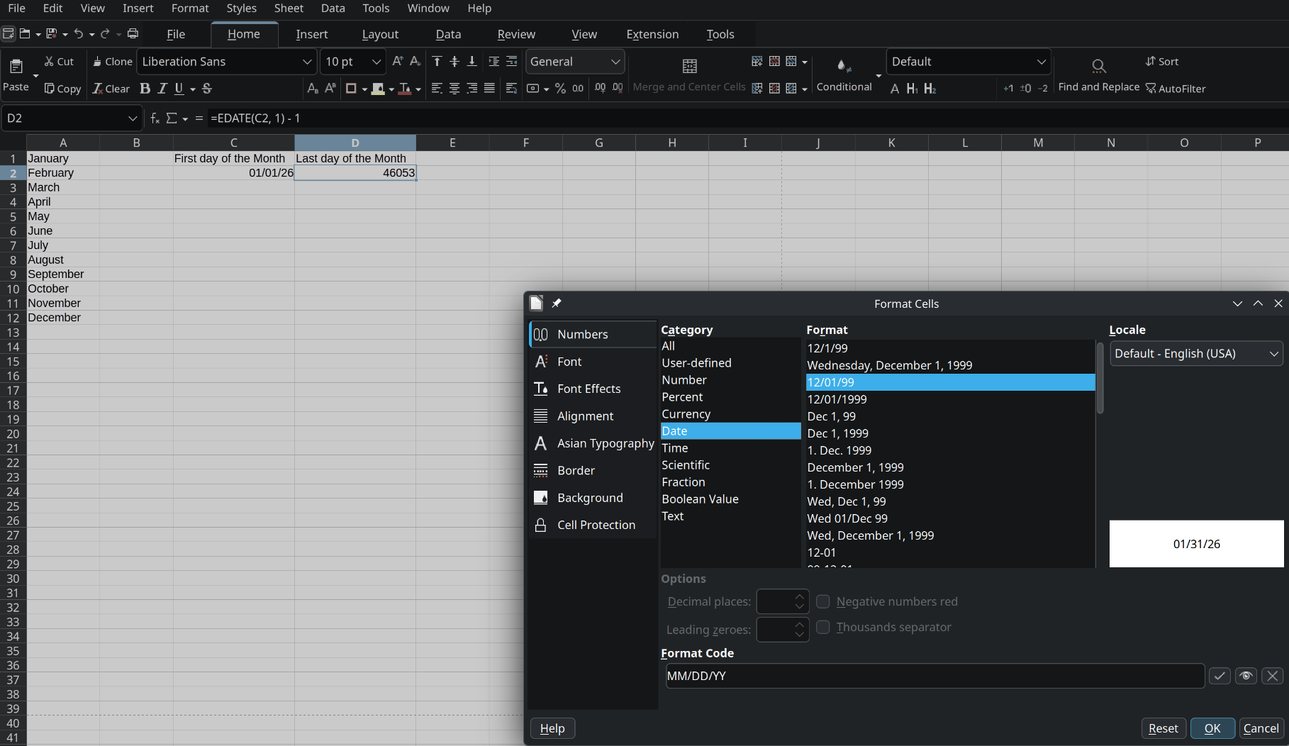
   • In cell C1, type label: First Day of the Month.

   • In cell C2, enter formula to calculate the start date of the active month:

     =DATE($'Month Calendar'.G1, MATCH($'Month Calendar'.A1, A1:A12, 0), 1)
     

   • In cell D1, type label: Last Day of the Month.

   • In cell D2, enter formula to calculate the end date of the active month:

     =EDATE(C2, 1) - 1
     

   • Make sure the format of the cell is set to Date ->Format -(12/01/99)

1. Select Calendar Date Ranges:
   • Switch back to the Month Calendar sheet.
   • Select all date header rows while holding Ctrl: A3:G3, A5:G5, A7:G7, A9:G9, A11:G11, A13:G13
2. Create and Customize the “Faded” Cell Style:
   • Press F11 (or go to Styles -> Manage Styles) to open the Styles sidebar.
   • Click the Cell Styles icon at the top of the sidebar.
   • Right-click Default (or any empty space in the style list) and select New… (or right-click Faded and select Modify… if it already exists).
   • In the General tab, enter Faded in the Name box.
   • In the Font Effects tab, set Font color to a light muted shade (e.g., Light Gray or Gray 4).
   • Click OK to save the new style.
3. Configure Conditional Formatting Rules: Monthly Calendar sheet
   • Go to Format -> Conditional -> Condition… -> More Rules
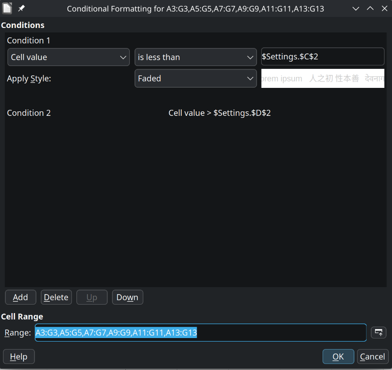
   • Set Condition 1:
     • Cell value -> is less than -> $Settings.$C$2
     • Apply Style: Select Faded

• Click Add to create Condition 2:
  • Cell value -> is greater than -> $Settings.$D$2
  • Apply Style: Select Faded

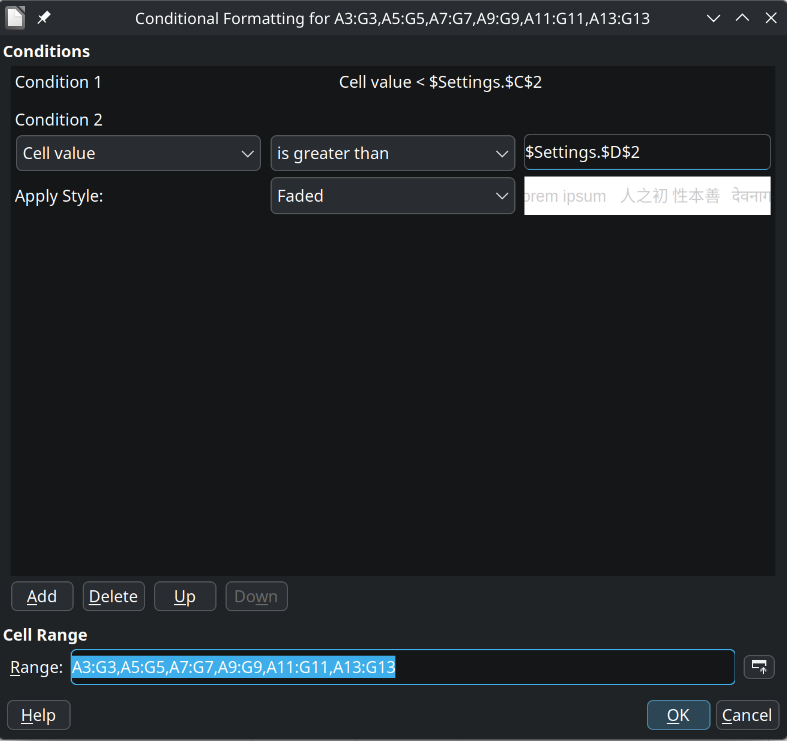
• Confirm the target Cell Range is set to: A3:G3,A5:G5,A7:G7,A9:G9,A11:G11,A13:G13
• Click OK. Days belonging to the previous or next month will now automatically display in grayed-out/faded text.

---

Step 8: Add & Highlight National Holidays (Optional)

1. Create Holiday Table in Settings Sheet:
   • Switch to the Settings sheet.
   • In Column F (cells F2:F20), enter your list of national holiday dates (e.g., 2026-01-01, 2026-07-04, 2026-12-25).
   • In Column G (cells G2:G20), enter the corresponding holiday names (e.g., New Year's Day, Independence Day, Christmas).
2. Create a “Holiday” Cell Style:
   • Press F11 to open the Styles sidebar.
   • Right-click in the style list and select New….
   • In the Organizer tab, set Name to Holiday.
   • In the Background tab, pick a soft accent color (e.g., Light Red or Soft Yellow).
   • In the Font Effects / Font tab, apply bold text or a dark accent color.
   • Click OK.
3. Configure Conditional Formatting Rule for Holidays:
   • Switch back to the Month Calendar sheet.
   • Select all calendar date cells (A3:G3, A5:G5, A7:G7, A9:G9, A11:G11, A13:G13).
   • Go to Format -> Conditional -> Condition… (or Manage…).
   • Click Add to create a new rule:
     • Change condition type from Cell value to Formula is.

     • Enter formula:

       COUNTIF($Settings.$F$2:$F$20, A3) > 0
       

     • Apply Style: Select Holiday.
   • Click OK. Any date on the calendar matching a date in your holiday table will now automatically highlight.
4. Automatically Display Holiday Names in Event Rows (Optional):
   • To show the holiday title directly in the box under each date row, enter the corresponding VLOOKUP formula in Column A for each event row:

     • Cell A4 (under Week 1 date A3):

       =IFERROR(VLOOKUP(A3, $Settings.$F$2:$G$20, 2, FALSE), "")
       

     • Cell A6 (under Week 2 date A5):

       =IFERROR(VLOOKUP(A5, $Settings.$F$2:$G$20, 2, FALSE), "")
       

     • Cell A8 (under Week 3 date A7):

       =IFERROR(VLOOKUP(A7, $Settings.$F$2:$G$20, 2, FALSE), "")
       

     • Cell A10 (under Week 4 date A9):

       =IFERROR(VLOOKUP(A9, $Settings.$F$2:$G$20, 2, FALSE), "")
       

     • Cell A12 (under Week 5 date A11):

       =IFERROR(VLOOKUP(A11, $Settings.$F$2:$G$20, 2, FALSE), "")
       

     • Cell A14 (under Week 6 date A13):

       =IFERROR(VLOOKUP(A13, $Settings.$F$2:$G$20, 2, FALSE), "")
       

   • For each event row, select the Column A cell and drag/copy the fill handle across to Column G (B4:G4, B6:G6, B8:G8, etc.).
   • When a holiday occurs, its name will automatically populate in the event space directly below its date!

---

Step 9: Create an Annual Master View (3x4 Grid Layout & 1-Page Print Setup) Optional

1. Add a New Worksheet Tab:
   • Right-click the sheet tab list at the bottom and select Insert Sheet….
   • Name the new worksheet Annual View.
2. Set Up Master Year Header:
   • In cell A1, enter the label: Year.
   • In cell B1, enter the target year: 2026 (or =YEAR(TODAY())).
   • Format A1:B1: Font size 14pt, Bold, font color Dark Blue (#1F497D), left-aligned.
3. Adjust Column Widths & Row Heights:
   • Set Day Column Widths: Select all 21 day columns across the three month blocks—Columns A:G, I:O, and Q:W—right-click the column headers -> Column Width… -> set to 0.45” (or 1.15 cm).
   • Set Spacer Column Widths: Select spacer Columns H and P -> right-click -> Column Width… -> set to 0.25” (or 0.6 cm).
   • Set Row Heights:
     • Year Header Row (Row 1): Set height to 0.25” (0.65 cm).
     • Month Title Rows (Rows 3, 12, 21, 30): Set height to 0.25” (0.65 cm).
     • Weekday Header Rows (Rows 4, 13, 22, 31): Set height to 0.20” (0.5 cm).
     • Date Grid Rows (Rows 5–10, 14–19, 23–28, 32–37): Set height to 0.20” (0.5 cm).
     • Spacer Rows (Rows 2, 11, 20, 29): Set height to 0.15” (0.4 cm).
4. Construct the 3x4 Month Grid Structure (7-Column Mini Blocks):
   • Organize the 12 calendar months into 3 columns across and 4 rows down:
     • Column 1 Block (Spreadsheet Cols A–G):
       • January: Title merged A3:G3, Day Headers A4:G4, Date Grid A5:G10.
       • April: Title merged A12:G12, Day Headers A13:G13, Date Grid A14:G19.
       • July: Title merged A21:G21, Day Headers A22:G22, Date Grid A23:G28.
       • October: Title merged A30:G30, Day Headers A31:G31, Date Grid A32:G37.
     • Column 2 Block (Spreadsheet Cols I–O, Column H spacer):
       • February (I3:O10), May (I12:O19), August (I21:O28), November (I30:O37).
     • Column 3 Block (Spreadsheet Cols Q–W, Column P spacer):
       • March (Q3:W10), June (Q12:W19), September (Q21:W28), December (Q30:W37).
5. Configure Font & Text Formatting for Mini Month Blocks:
   • Month Titles (e.g., A3:G3 merged, I3:O3 merged, Q3:W3 merged): Set font to 11pt Bold, Dark Blue text (#1F497D), centered horizontally and vertically. Set Date Format Code to MMMM.
   • Weekday Headers (e.g., A4:G4, I4:O4, Q4:W4): Set font to 8pt Bold, Gray text (#595959), centered horizontally. Enter single-letter day abbreviations (S, M, T, W, T, F, S).
   • Date Grid Cells (e.g., A5:G10, I5:O10, Q5:W10): Set font to 8pt Regular, centered horizontally and vertically. Set Date Format Code to d.
6. Configure Mini Month Block Formulas (Detailed Cell-by-Cell Example for January):
   • Month Title Header (Cell A3 or merged A3:G3):

     =DATE($B$1, 1, 1)
     

   • Weekday Headers (Row 4): Enter day abbreviations across cells A4:G4: | Cell | A4 | B4 | C4 | D4 | E4 | F4 | G4 | | —— | —— | —— | —— | —— | —— | —— | —— | | Label | S | M | T | W | T | F | S |

   • Week 1 First Sunday Calculation (Cell A5):

     =DATE($B$1, 1, 1)-(WEEKDAY(DATE($B$1, 1, 1))-1)
     

   • Horizontal & Vertical Grid Increments:
     • Horizontal Addition (+1): In cell B5, enter =A5+1. Copy/drag across C5:G5 (=B5+1, =C5+1, etc.) to populate Monday–Saturday.
     • Vertical Addition (+7): In cell A6 (Sunday of Week 2), enter =A5+7. Copy/drag row 5’s horizontal formulas across B6:G6.
     • Remaining Weeks: Copy row 6 formulas down through rows 7–10 to complete January’s grid.
7. Replicate Block Formulas Across All 12 Months:
   • Repeat the mini month block formulas across the remaining 11 month blocks, updating the month index parameter in =DATE($B$1, MONTH_NUMBER, 1)-(WEEKDAY(DATE($B$1, MONTH_NUMBER, 1))-1) for each month position (1 through 12).
8. Apply Conditional Formatting to Fade Neighboring Month Dates:
   • To automatically gray out dates belonging to preceding or subsequent months in each mini grid:
     1. Select the date cell range for a month block (e.g., A5:G10 for January).
     2. Go to Format -> Conditional -> Condition…
     3. Set Condition 1 (Fade preceding month dates):
        • Cell value -> is less than -> DATE($B$1, Month_Number, 1)
        • Apply Style: Select Faded
     4. Click Add to create Condition 2 (Fade subsequent month dates):
        • Cell value -> is greater than -> EDATE(DATE($B$1, Month_Number, 1), 1) - 1
        • Apply Style: Select Faded
     5. Click OK.

---

Values for All 12 Months

For each month block across the 3x4 grid, you change the second parameter in DATE($B$1, Month_Number, 1) to match the month number (1 for Jan, 2 for Feb, up to 12 for Dec):

Month	Date Cell Range	Condition 1: is less than	Condition 2: is greater than
1. January	A5:G10	DATE($B$1, 1, 1)	EDATE(DATE($B$1, 1, 1), 1) - 1
2. February	I5:O10	DATE($B$1, 2, 1)	EDATE(DATE($B$1, 2, 1), 1) - 1
3. March	Q5:W10	DATE($B$1, 3, 1)	EDATE(DATE($B$1, 3, 1), 1) - 1
4. April	A14:G19	DATE($B$1, 4, 1)	EDATE(DATE($B$1, 4, 1), 1) - 1
5. May	I14:O19	DATE($B$1, 5, 1)	EDATE(DATE($B$1, 5, 1), 1) - 1
6. June	Q14:W19	DATE($B$1, 6, 1)	EDATE(DATE($B$1, 6, 1), 1) - 1
7. July	A23:G28	DATE($B$1, 7, 1)	EDATE(DATE($B$1, 7, 1), 1) - 1
8. August	I23:O28	DATE($B$1, 8, 1)	EDATE(DATE($B$1, 8, 1), 1) - 1
9. September	Q23:W28	DATE($B$1, 9, 1)	EDATE(DATE($B$1, 9, 1), 1) - 1
10. October	A32:G37	DATE($B$1, 10, 1)	EDATE(DATE($B$1, 10, 1), 1) - 1
11. November	I32:O37	DATE($B$1, 11, 1)	EDATE(DATE($B$1, 11, 1), 1) - 1
12. December	Q32:W37	DATE($B$1, 12, 1)	EDATE(DATE($B$1, 12, 1), 1) - 1

• Updating the master year in cell B1 automatically updates all 12 mini month blocks and their conditional formatting across the entire 3x4 grid!

---

Values for All 12 Months (Fading & Holiday Highlighting)

For each month block across the 3x4 grid, apply Conditions 1 & 2 for fading outside dates, plus Condition 3 for highlighting national holidays from your $Settings.$F$2:$F$20 list:

Month	Date Cell Range	Condition 1: is less than	Condition 2: is greater than	Condition 3: Formula is
1. January	A5:G10	DATE($B$1, 1, 1)	EDATE(DATE($B$1, 1, 1), 1) - 1	COUNTIF($Settings.$F$2:$F$20, A5) > 0
2. February	I5:O10	DATE($B$1, 2, 1)	EDATE(DATE($B$1, 2, 1), 1) - 1	COUNTIF($Settings.$F$2:$F$20, I5) > 0
3. March	Q5:W10	DATE($B$1, 3, 1)	EDATE(DATE($B$1, 3, 1), 1) - 1	COUNTIF($Settings.$F$2:$F$20, Q5) > 0
4. April	A14:G19	DATE($B$1, 4, 1)	EDATE(DATE($B$1, 4, 1), 1) - 1	COUNTIF($Settings.$F$2:$F$20, A14) > 0
5. May	I14:O19	DATE($B$1, 5, 1)	EDATE(DATE($B$1, 5, 1), 1) - 1	COUNTIF($Settings.$F$2:$F$20, I14) > 0
6. June	Q14:W19	DATE($B$1, 6, 1)	EDATE(DATE($B$1, 6, 1), 1) - 1	COUNTIF($Settings.$F$2:$F$20, Q14) > 0
7. July	A23:G28	DATE($B$1, 7, 1)	EDATE(DATE($B$1, 7, 1), 1) - 1	COUNTIF($Settings.$F$2:$F$20, A23) > 0
8. August	I23:O28	DATE($B$1, 8, 1)	EDATE(DATE($B$1, 8, 1), 1) - 1	COUNTIF($Settings.$F$2:$F$20, I23) > 0
9. September	Q23:W28	DATE($B$1, 9, 1)	EDATE(DATE($B$1, 9, 1), 1) - 1	COUNTIF($Settings.$F$2:$F$20, Q23) > 0
10. October	A32:G37	DATE($B$1, 10, 1)	EDATE(DATE($B$1, 10, 1), 1) - 1	COUNTIF($Settings.$F$2:$F$20, A32) > 0
11. November	I32:O37	DATE($B$1, 11, 1)	EDATE(DATE($B$1, 11, 1), 1) - 1	COUNTIF($Settings.$F$2:$F$20, I32) > 0
12. December	Q32:W37	DATE($B$1, 12, 1)	EDATE(DATE($B$1, 12, 1), 1) - 1	COUNTIF($Settings.$F$2:$F$20, Q32) > 0

• Updating the master year in cell B1 automatically updates all 12 mini month blocks and their conditional formatting across the entire 3x4 grid!